Start with Bezier Curves
Let’s draw a smooth spline today!
The simplest ways to draw a line between is to draw a straight line between them.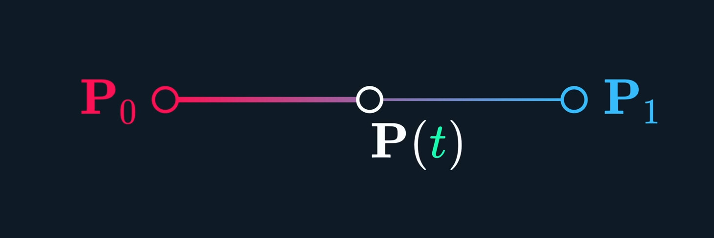
We input a percentage to this function that detmine har far between the two points.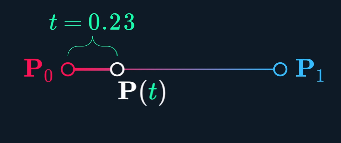
This is the most common type of blending, we call it #lerp
$$P (t) = (1-t) P_0 + t P_1\tag{Lerp}$$
We add one point, we ues the extra same lerp function, to blend these points on each line, and use the third line to interpolated points to get one curve.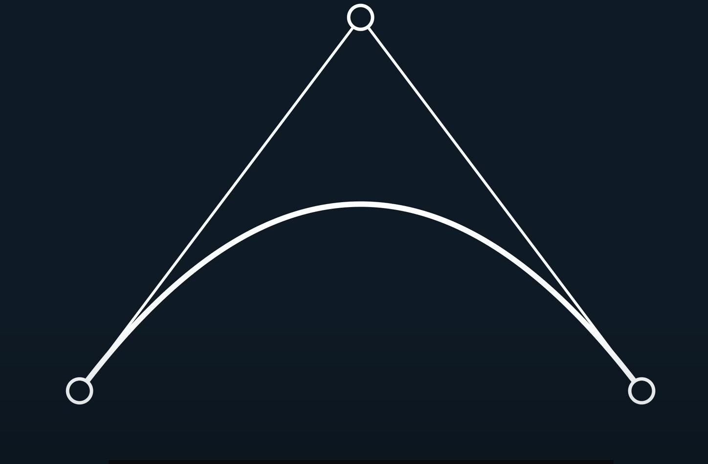
This is the magic of Bezier curves! Using Only linear interpolation to get a smooth curve.
This one is particular, is Quadratic Bezier Curve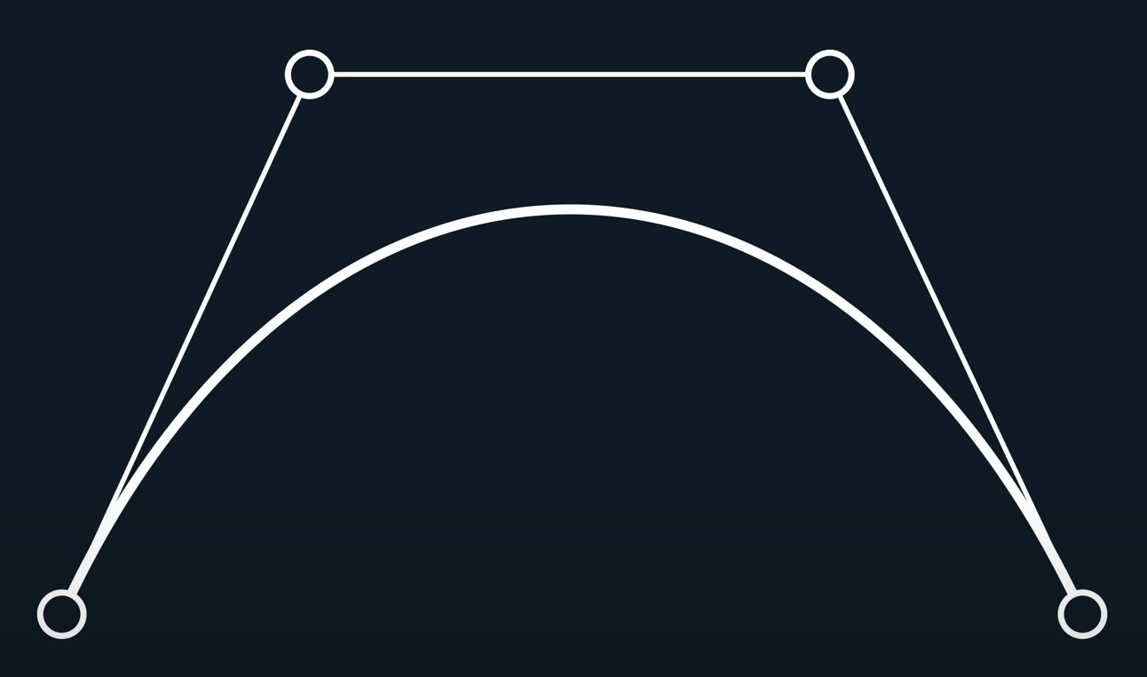
The same way, we add another point, and we get the cubic Bezier Curve. Cubic Bezier Curve is the most common curve so far. Almost every font and vector graphics tool, is using the cubic bezier curve.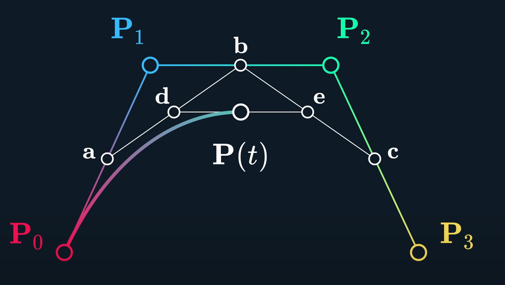
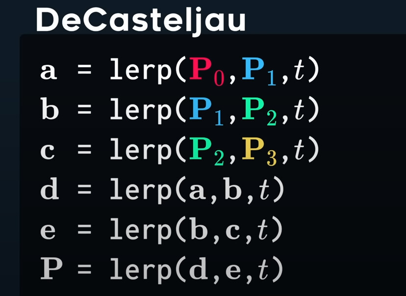
This method of recursively lerping between is called DeCasteljau. You just lerp until you run out of things to lerp.
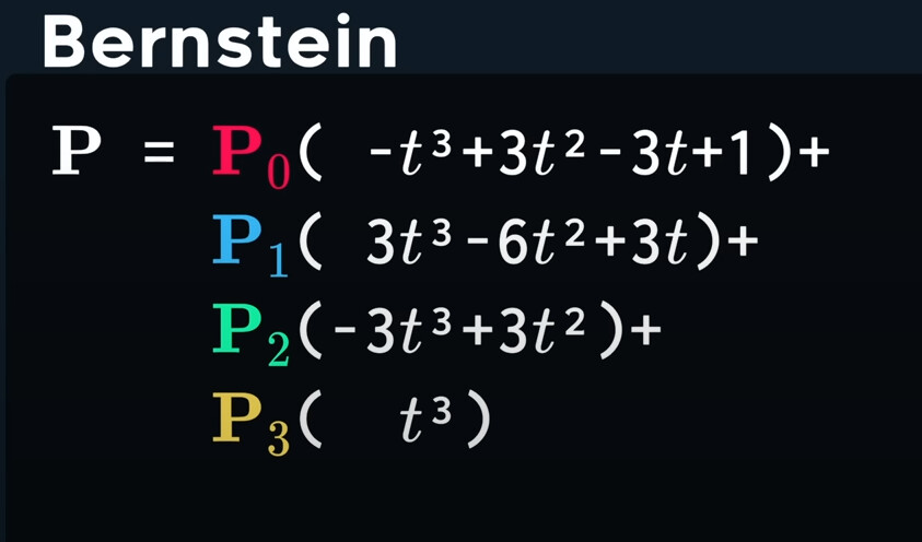
These polynormaials act as influences of each control point.
Influence change with curve goes. This is a special type of weighted sum, called a convex conmination.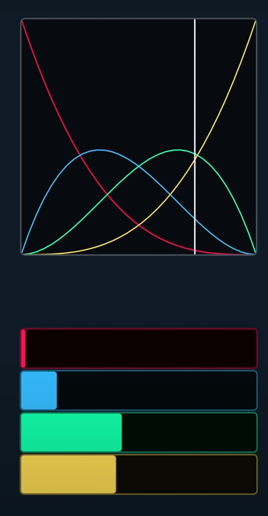
We can also think that it is the combination of vectors.
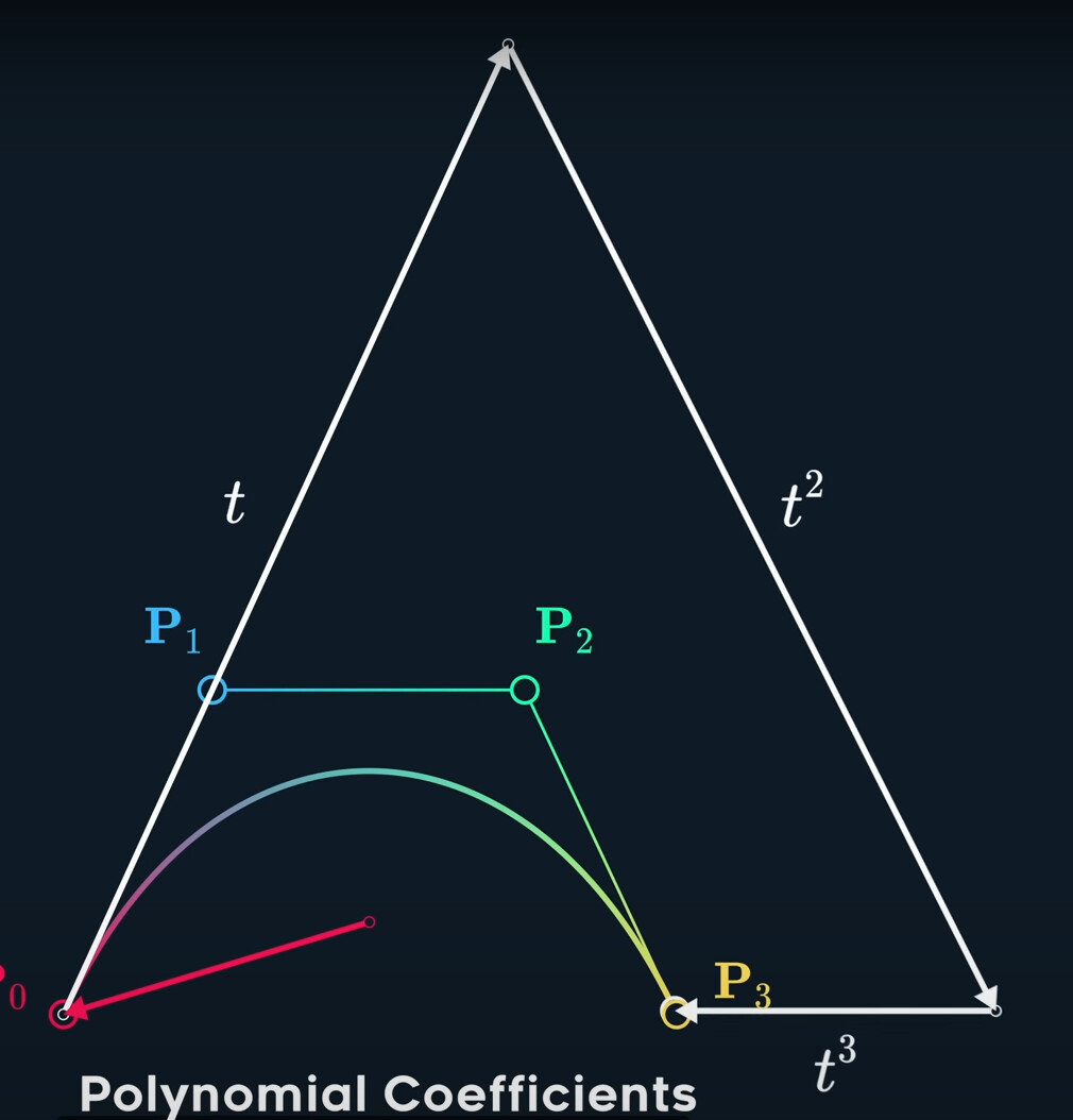
The same result, they have different geometric interpretations and performance characteristics.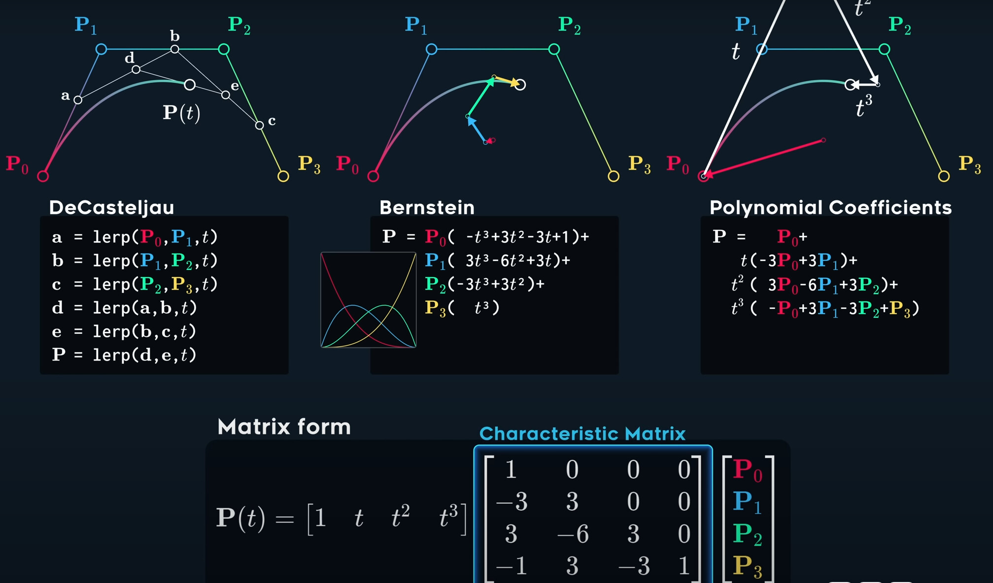
But in this condition, we have no local control. Every movement of every point affects the entire curve.
Besides, it doesn’t pass through most points, so it is difficult to make a specific paths of the shape you want.
Finally, the number of control points is numberically unstable or very expensive to calculate.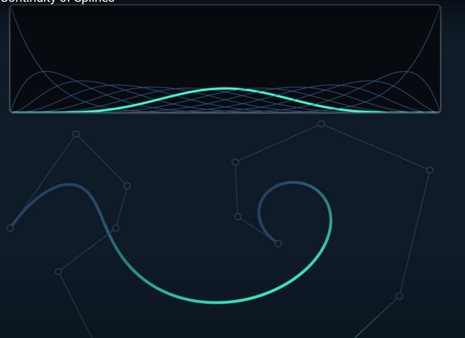
So we need to find the answer that we can control shapes without affecting every single other point in the curve.
We consider cubic bezier curve again, we combine some curves together, sharing the point.
Traversing this path requires some extra work. Because input t-value was traditionally from 0 to 1, acting as a kind of percentage along the curve.
In this condition, we can easily map each curve to each whole number.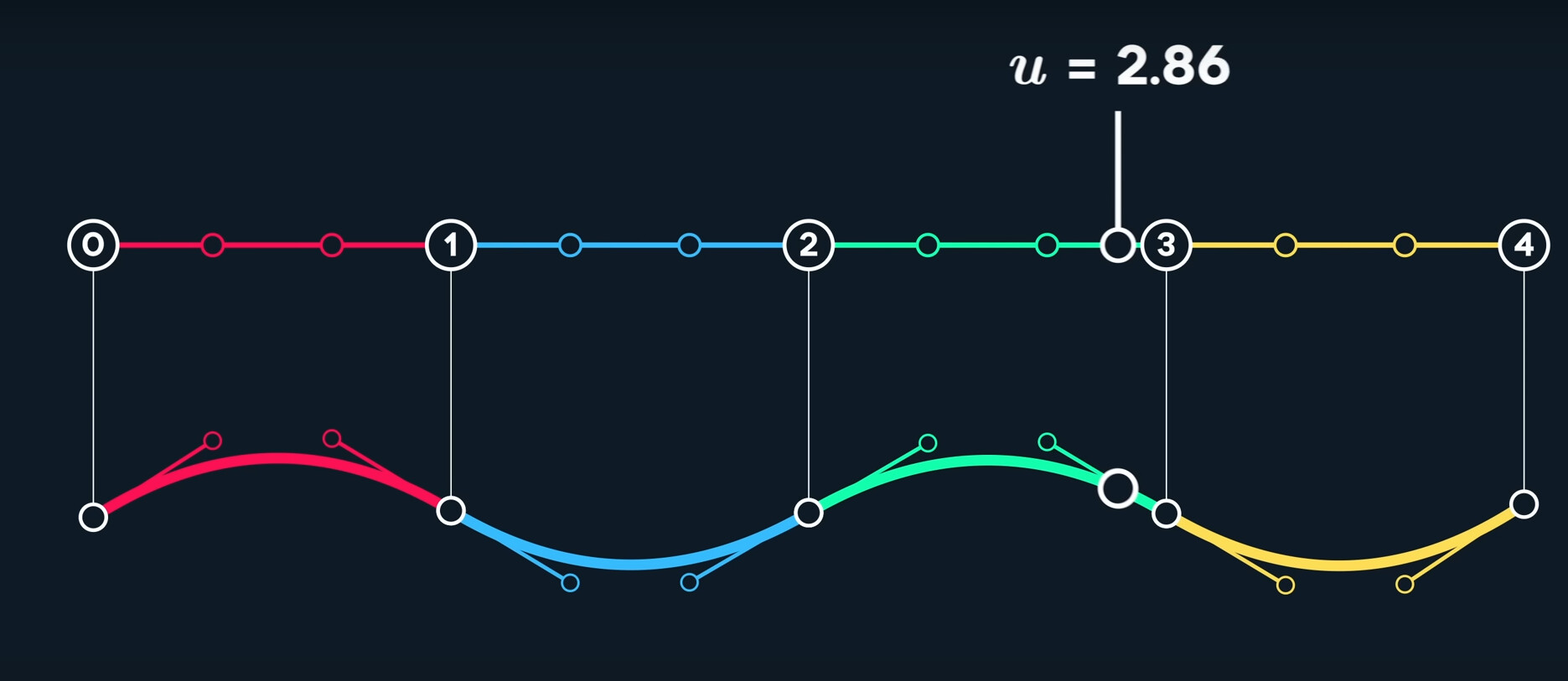
The input u-value, is in a one-dimensional space called parameter space. The points we define are called control points.
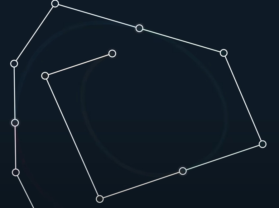
In this condition, where each curve is effectively using its own math function. These curves meet end to end at points called joins or knots.
Each curve is then assigned an interval in the input parameter space, that helps us associate any given input u value to a curve. The values here are called knot values.

We map the basic functions into our parameter space,
It is clear that with cubic bezier spline, we’ve regained local control. We just effecitively sampling one cubic bezier, so it doesn’t get any more expensive.
It’s now interpolating every third point, so it is easier to create whatever shape we want.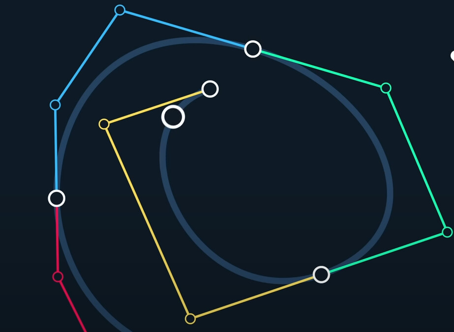
It’s the reason why cubic bezier curve are so popular, it really gives you a huge amount of control.
There are three common configurations about hte curve joins, also called tangent points.
One is split tangents, also known as broken tangents, we can use to make sharp conners.
The second one is where you align three points around the curve join, which ensure the two curves are tangent with each other at that join.
Finnally, we can also mirror the tangent points around the join, making them not only aligned, but also the same distance from their shared control point.
With all these tools in mind, we can now easily create paths, and animate objects on it.
Continuity
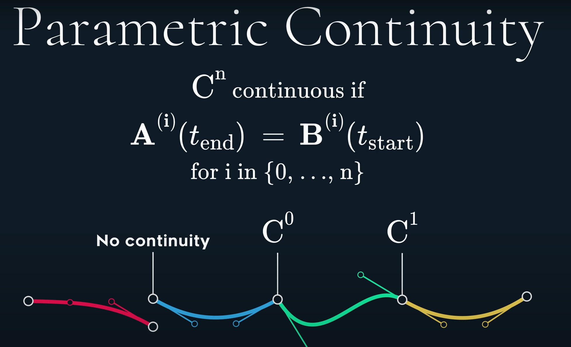
Continuity is a measure of how “connected” the curve are.
Continuity means is that posision changes continuously, there’s no sudden jump, or discontinuity in this path.
If we want to analyze change, it’s worth looking into derivatives.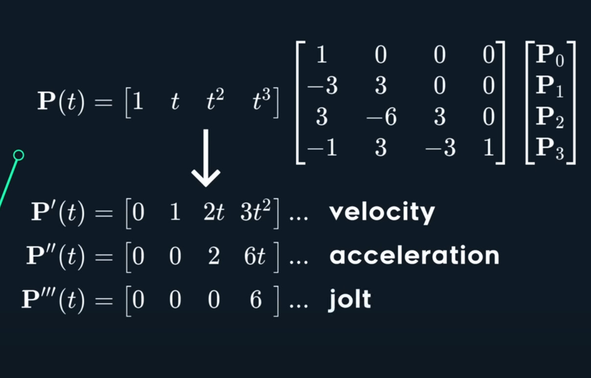
The velocity graph is discontinuous, it’s disconnected at every join.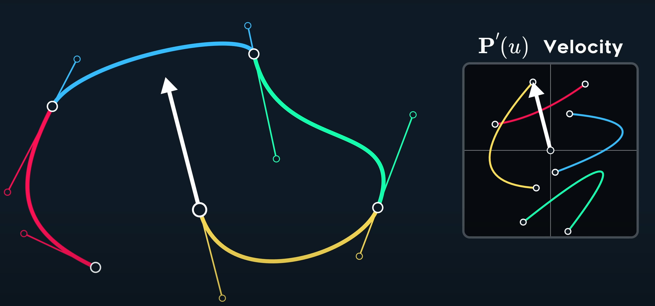
We change all join to mirro, the velcoity curve will be continuous.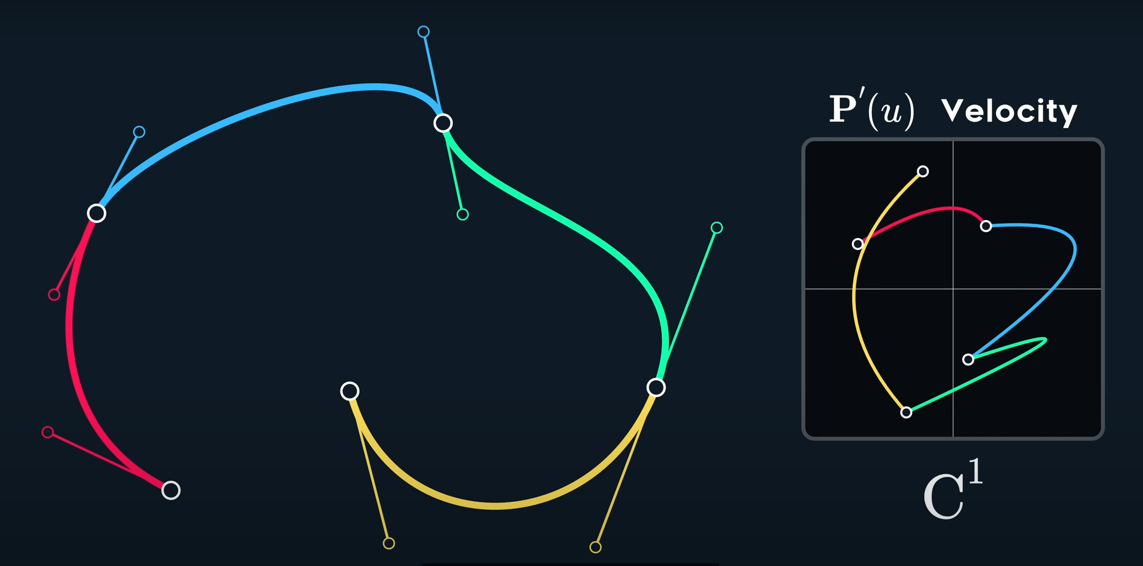
For C_2 continuity, we should control the acceleration in the join, in this condition, we successfully joined with C_2 continuity.
But we lose so much control of the curve, this can’t even be called a spline anymore.
To summarize, in a cubic bezier, when the tangent points are mirrored, we have C_1 continuity. When we have a broken join, the velcoity is no longer continuous, so it’s only continuous. When the curve is entirely disconnected, there’s no continuity at all.
Geometric Continuity
The change of speed has literally no effect on our tangent and normal, this is called tangent continuity, we’re going to call this G_1.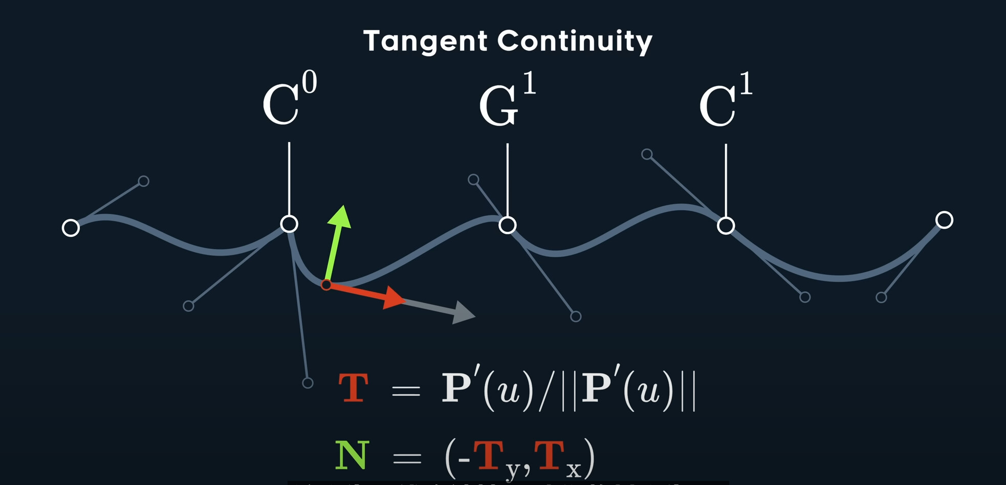
Regardless, so what is G_2?
To get the answer, we have enter the third dimension. If we look closely, we can see that something is wrong here.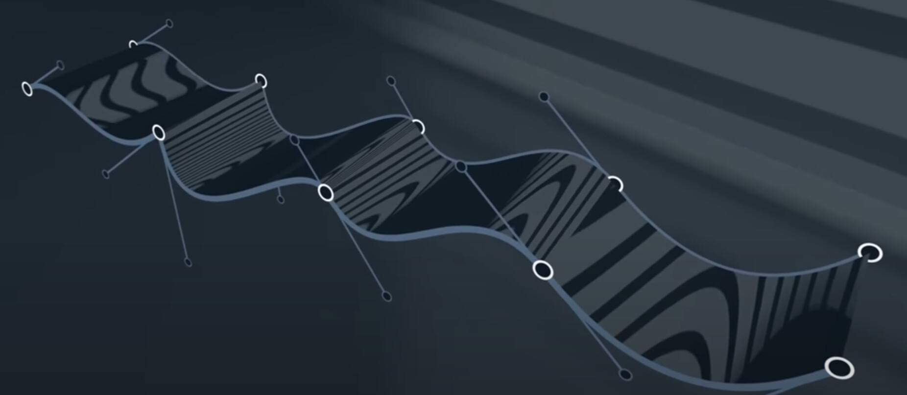
It is clear that how discontinuous this is.
This doesn’t just apply to bezier curves, so what happened?
We might notice they suddenly start and stop rotating at the joins.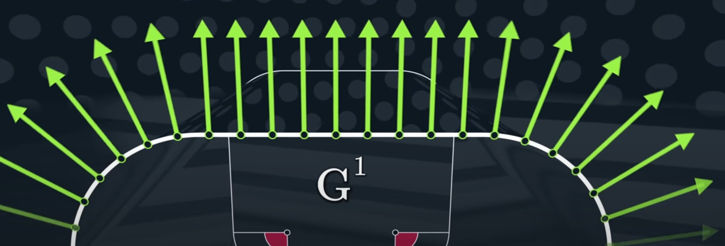
The angle of the tangent vector can illuminate this problem even more clearly. Notice how the angle is changing at a constant rate, they comes to a complete stop, and then it suddenly and immediately starts again.
In face, this is inherent to the nature of circles. We need a parameter-independent, or, speed-independent way to measure this, is where we need to talk about curvature.
Given a point on a curve, there’s a circle that describes the curvature at that point. This is called the osculating circle.
We can calculate the osculating by this way.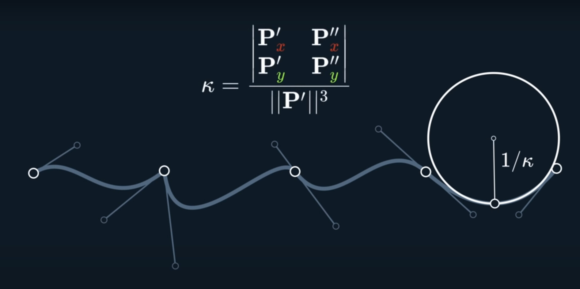
So what does the curvature look like across this spline?
A very popular way to analyze curvature is using this handy tool, known as a curvarue comb.
Did it solve our problem with shiny reflections?
It look yes.
We also needed curvarure continuity to get rid of the seam in the reflection. It will even pass the harder, dot pattern test.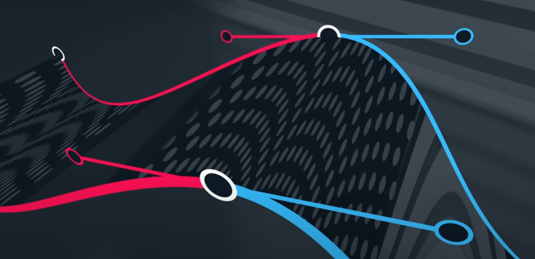
This is why $G^2$ continuity is very important in industrial design, as anything shiny will respond very strongle to the shape of the curves.
$G^1$ is when tangent are continuous, the curveture comb will also be aligned with itself across the normal of the curve.
$G^2$ is when curvarure is continuous. The curveture comb is now continuous in and of itself, as you can see, it connects surfaces that are $G^2$ or higher, sometimes called Class-A surfaces.
$G^3$ is when the rate fo change of curvature is continuous, the curvature comb will be in and of itself, tangent continuous.
Usually, we don’t go higher than $G^3$ as we get very diminshing returns in outcome and the math becomes significantly more unwiedly for each step.
So it is called Geometric Continuity
If you have two curves A and B, they are $G^n$ continuous, if a function g (t) exists, so that A (t) and B (g (t) ) are $C^n$ continuous.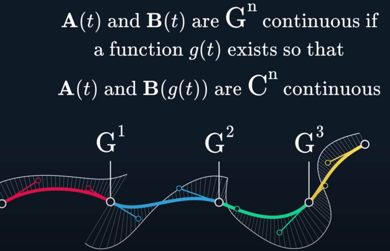
Let’s summarize, $C^0$ and $G^0$ are equivalent, and they are both positional continuity. It basically means your curves are simply connected in position.
$C^1$ is velcoity continuity, as in the first derivative is continuous, and the position is also continuous. In other words, it’s not enough for the velcoity to be continuous on its own, the previous derivatives have to be continuous as well.
$G^1$ is tangent continuity, which also requires that it has positional continuity. And, this same pattern continues.
$C^2$ is acceleration continuity, which also implies velcoity continuity, which also implies positional continuity.
$C^3$ is jolt continuity.
$G^2$ is curvature continuity, which again implies the previous ones.
Finally, we have $G^3$ which is incorrectly called “torsion” continuity, but it’s effectively refering to the rate of change of curvature.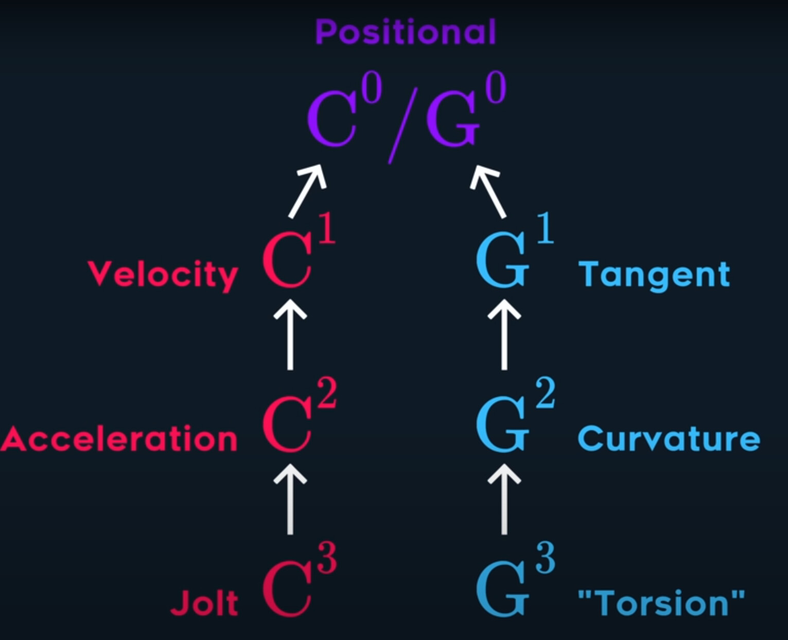
Now just like all the parametric continuities include all previous levels, and geometric continuity include all their previous levels.
There’s another connection here. $C^1$ continuity is also necessarily $G^1$ continuous.
Effectively, G-continuity is less strict than C-continuity. So the C-continuities actually imply their corresponding geometric continuity as well.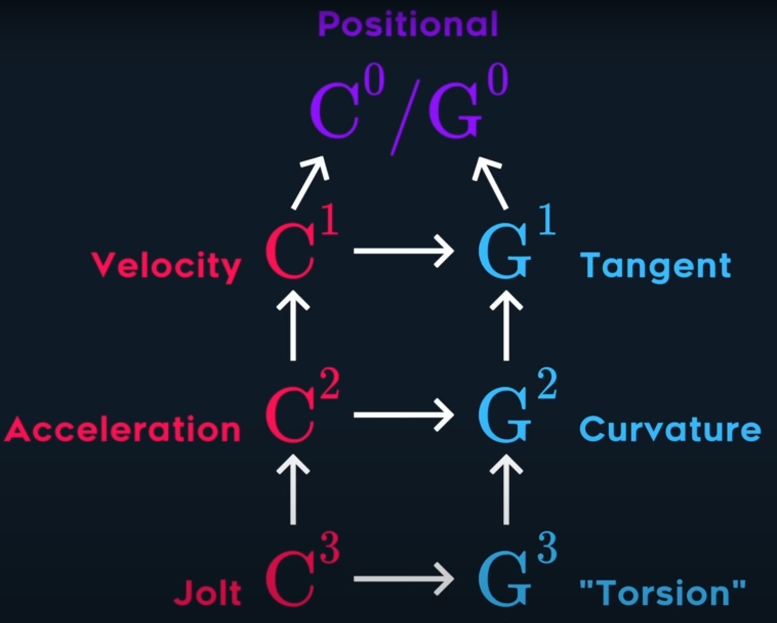
The rules only apply to regular curve. A regular curve is one where the velocity is never 0.
Such as this condition: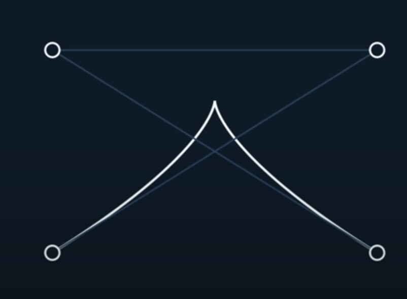
Bezier is strange, are they not?
They don’t really refer to anything specific, expect the start and the end point.
What if we can come up with another type fo spline, that makes more physical sense?
What if instead of supplying 4 points, we set the start and end point, as usual, but then we also set the start and end velcoities.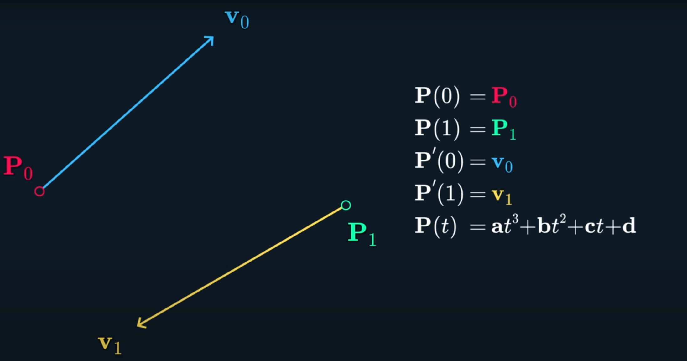

The cool thing about this one is that there’s no more arbitrary tangent points, it’s a spline that guarantees being at a specific place, with a cecrtain velcoity, at every control point.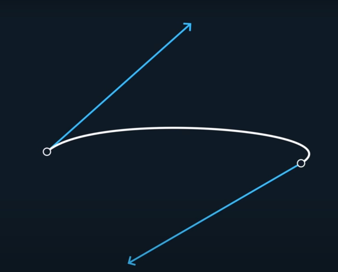
If we analyze the first derivative, the velocity, we can see it matches at every point along this spline, and it’s fully continuous.
This type of spline where you can supply explicit velocities at each point, actually has a name called Hermite Spline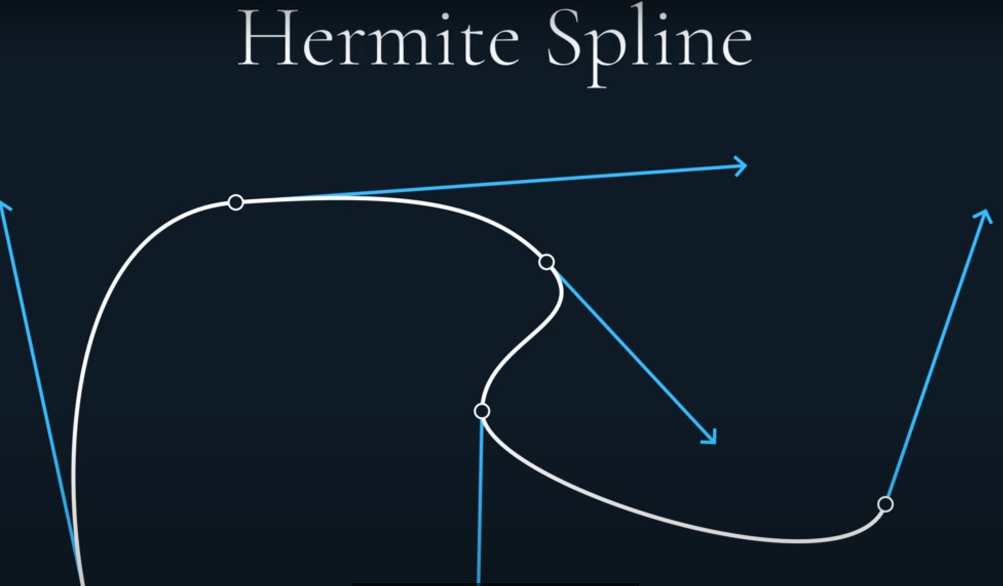
Anyway, as you can see, the hermite spline has explicit derivatives.
And since both sides of each curve join share the same velocity, it is also necessary $C^1$ continuous.
It’s also worth nothing, many hermite splines out there allow for two velocities per join.
It’s also interpolating, it’s passing through every point and every velocity.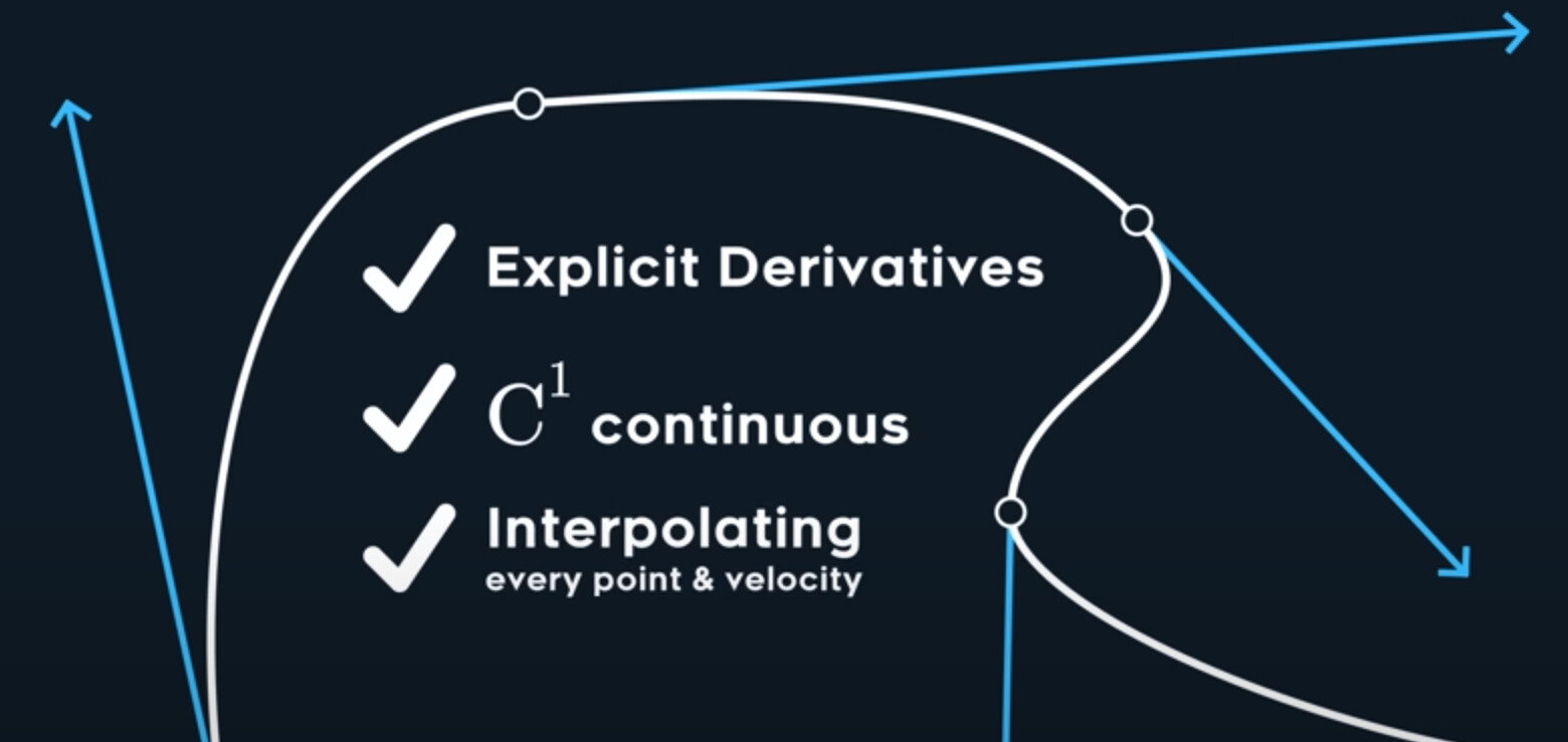
It is easy to change hermite spline to Bezier spline. If we divide each velocity by three, and add its origin, we will get the bezier tangent point, flip that to the other side, and will now have the bezier control point for the other side.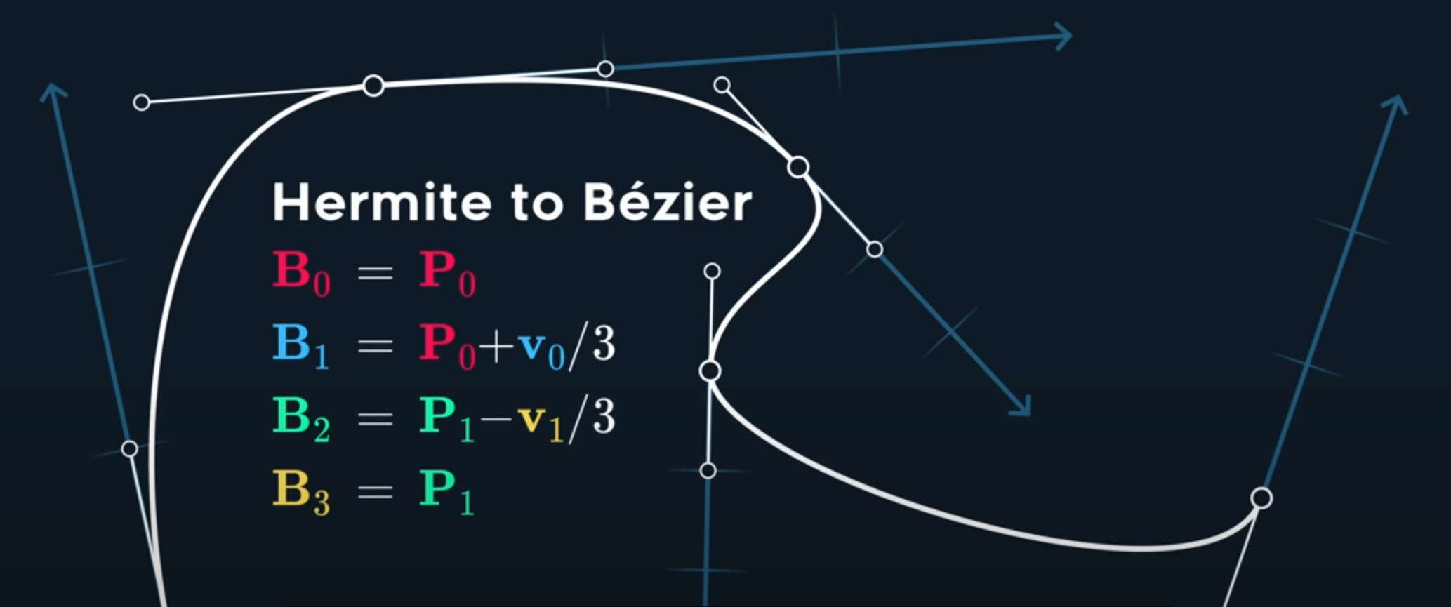
Linear Spline
Simply drawing straight lines between each point, it also has a few superpowers.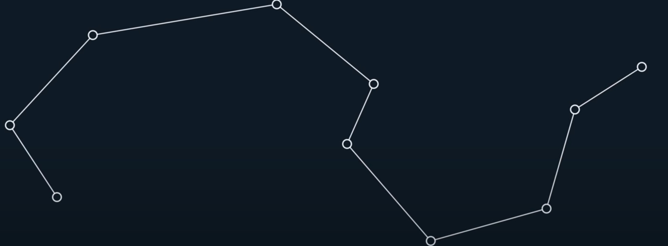
First, it passing through every control point.
Second , it’s one of the few splines where arc-length parameterization is easy! (Arc length parameterization is when you want to interpolate a curve with a constant speed, which is actually very complicated for almost all splines out there)
Third, it’s very cheap to evaluate! Here’s the formula, it’s just a lerp.
But unfortunally, it’s just $C^0$ continuous.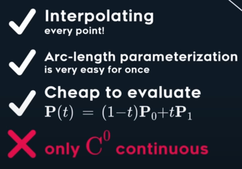
So we ask, is it possible to make a smoother spline?
This type fo spline with automatic tangents, a scale parameter and interpolating all points, is called a cardinal spline.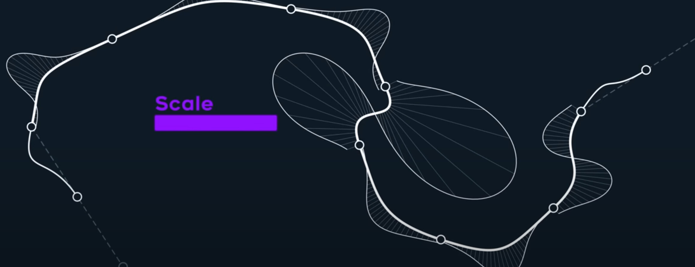
Here’s what its matrix form looks like!
For this reason, it’s called the catmull-rom spline. It pass through every point (except the endpoints that kind of need special handing). As for continuity, the curvature comb tells us it is $G^1$ continuous. Let’s also look at the parametric continuity.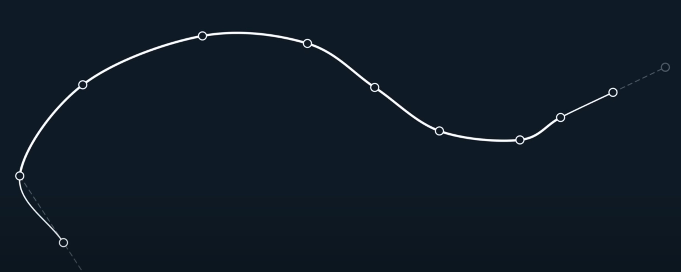
So the catmull-rom spline is $C^1$ continiuous, and there’s no need to specify tangents, it just works.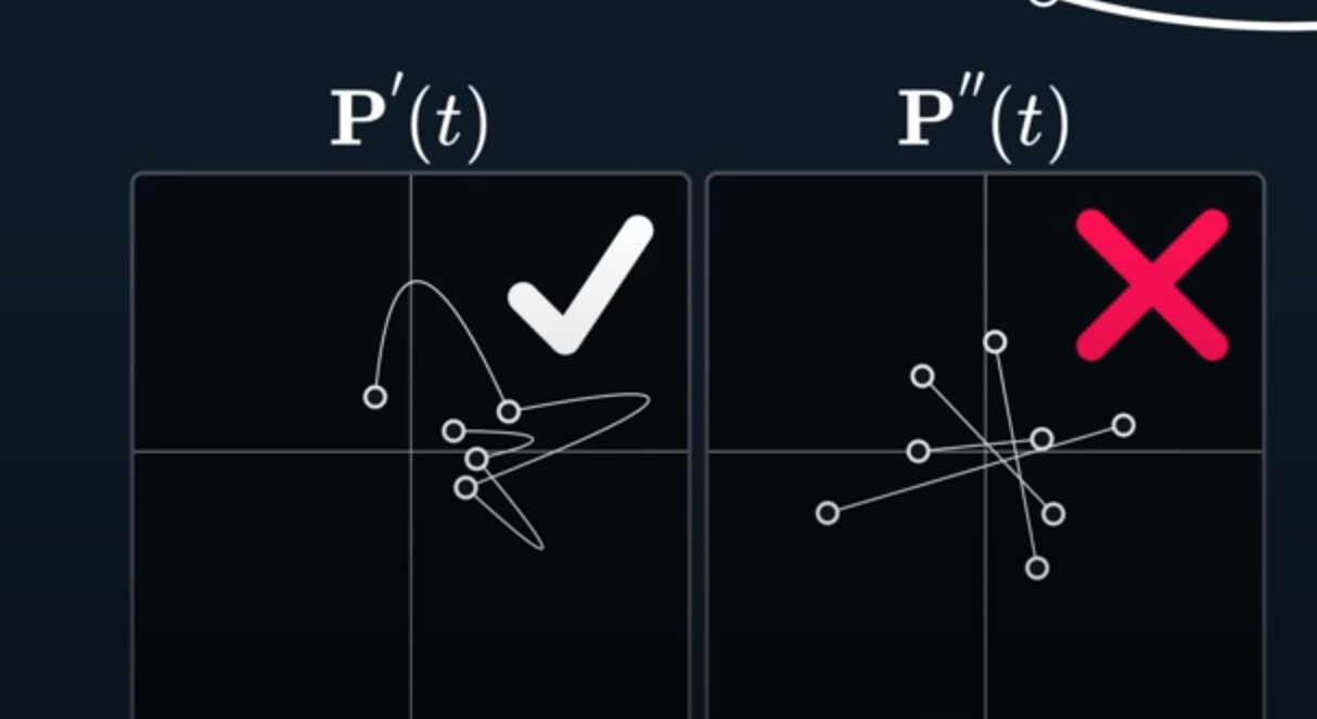

But it is still $C^1$ continuous.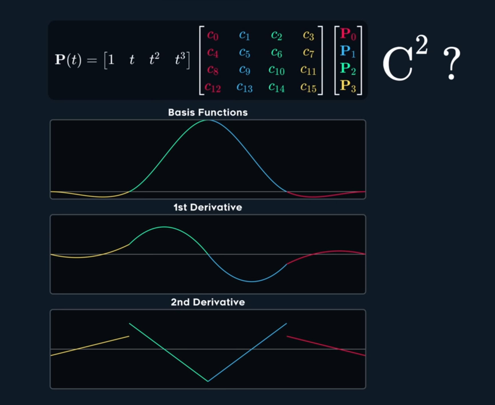
So this soft little spline, while it’s not interpolating like at all, it is actually $C^2$ continuous. The reason is possible because we sacrificed the interpolating property in favor of acceleration continuity.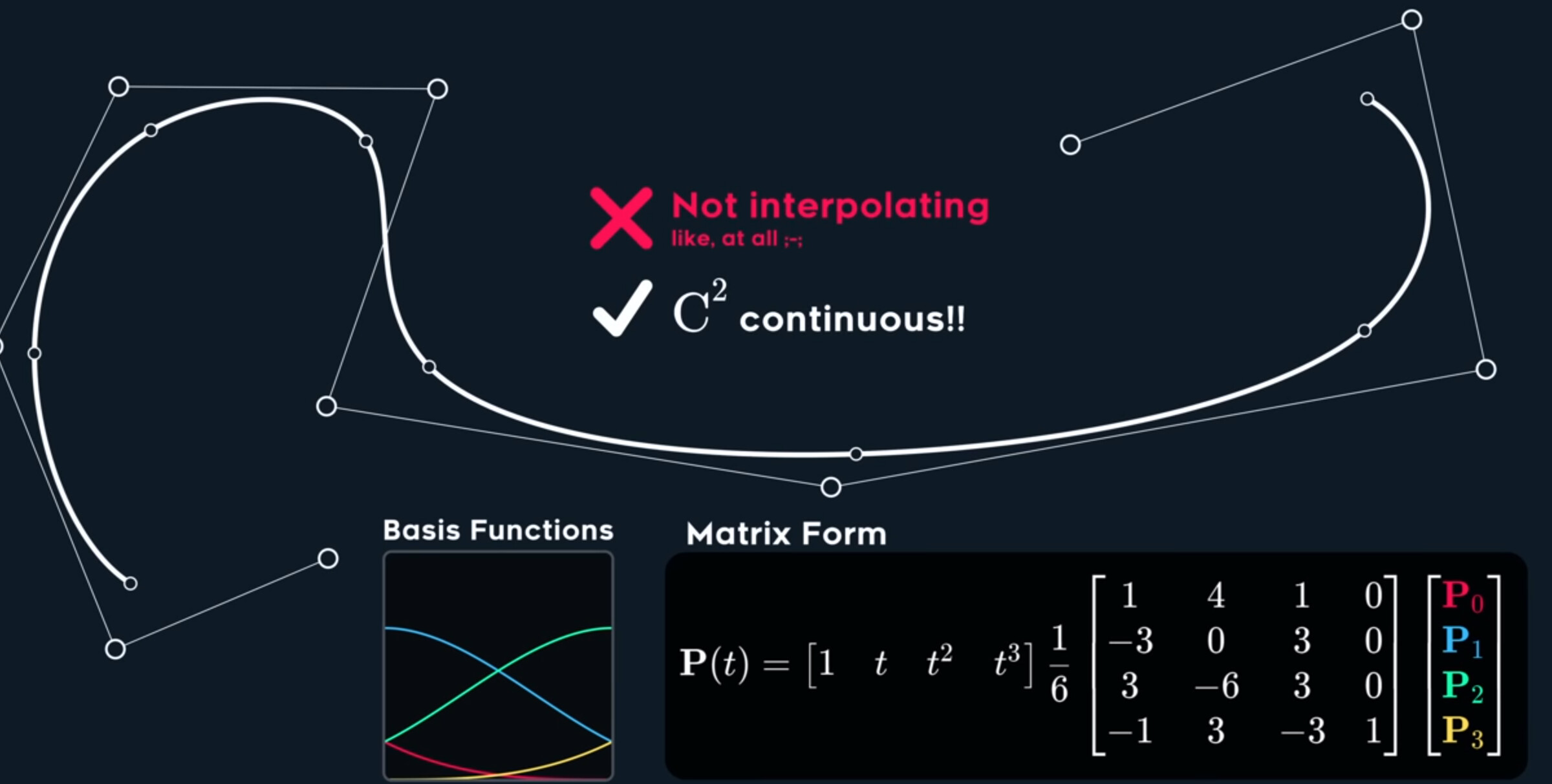
Of course, this spline have name, it’s called B-Spline, short for Basis Spline.
So what’s happening here, trick question aside, all of them can generate this specific curve. Beacuse all of these individual spline segments we’ve been talking about are actually very similar.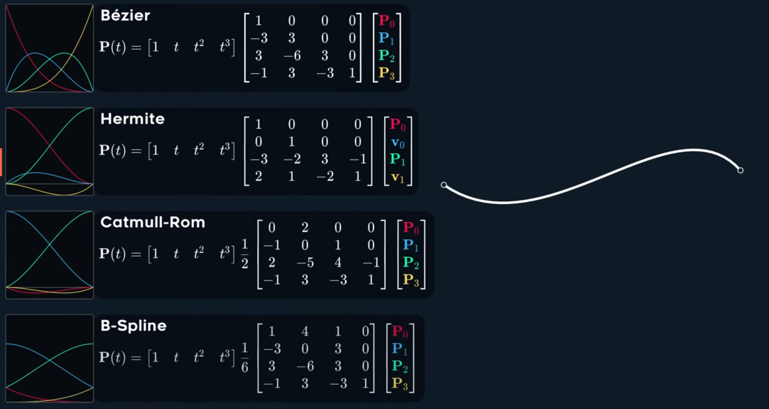
First, they are all uniform! They presume you want interpolate in a 0 to 1 range.
Second, they are all cubic polynomials. They all fit this formula.
So if they can generate the same curve, what’s even the point of different splines?
First, curves themselves are not splines! Thay are generated by splines. It’s all about how multiple curves, connect, and how smoothly they are able to do so. What splines really describe is a transformation of control points. Given some control points, you use a spline, to generate curves. If you swap out the spline, but keep the control points, you get different curves.
I want you to think of splines as curve geneartors, that make certain promises about continuity in the curve joins, and how it treats the input control points.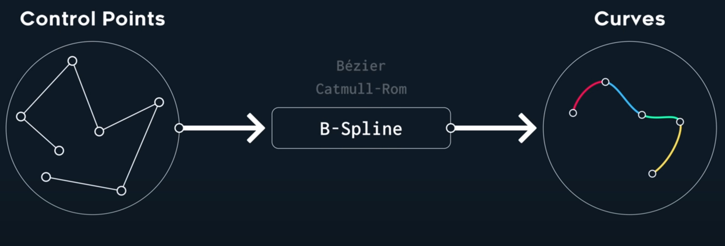
So it’s not just about the end result, but the process you used to get there . You know as they say, “it’s about the juorney, not the destination”
Summary
The Bezier spline gives us a huge amount of control. It lets us create sharp corners, in other words, intentional tangent discontonuities which is very useful when defining shapes like fonts or vector graphics, such as this heart.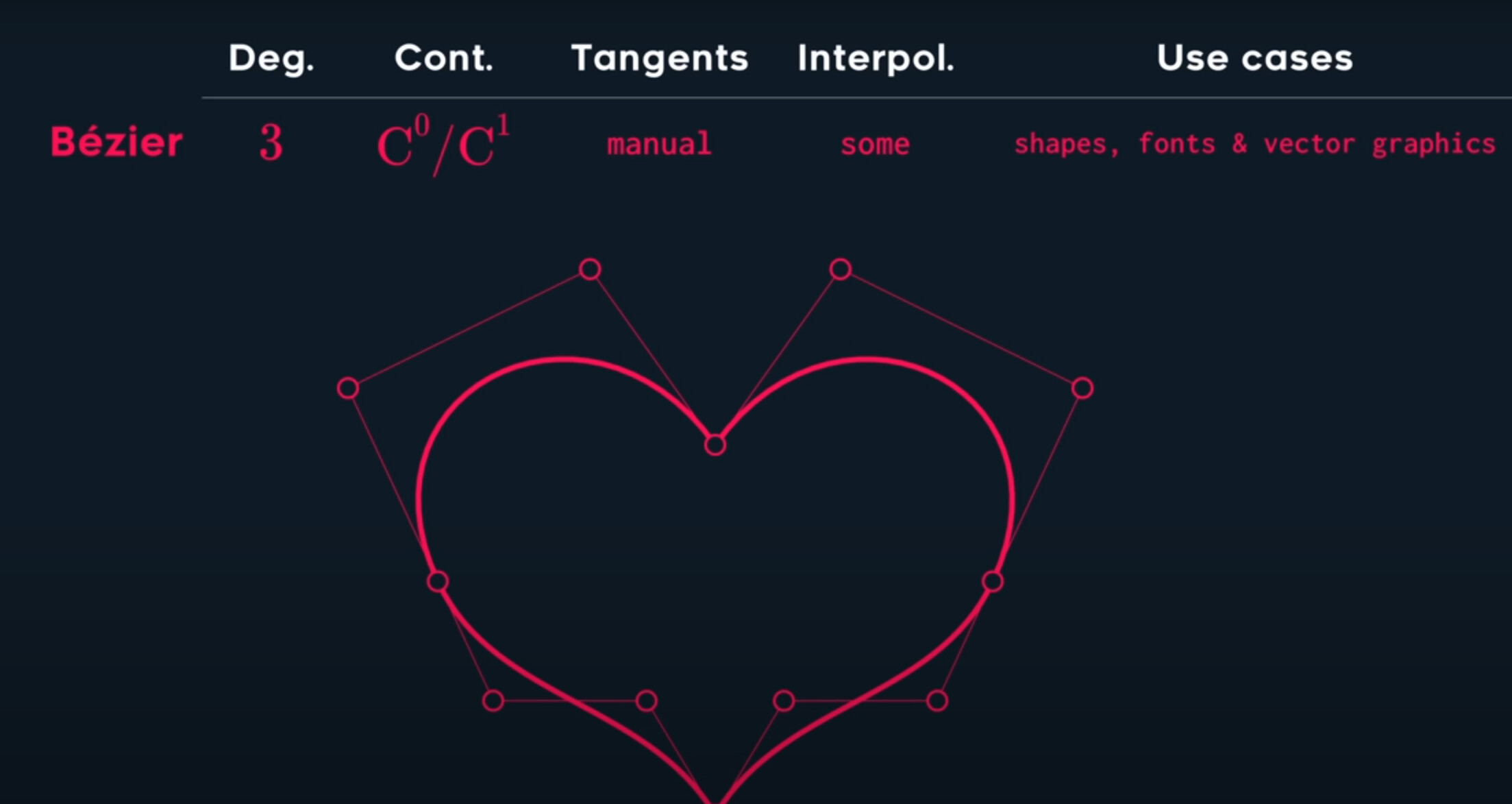
Hermite splines let us define explicit derivatives, guaranteeing it will pass through its points with specific velocities. This is the most common spline for animation, and its the basis for animation curve editor in Unity.
For example, let’s sya we want to animate a jumping square. We can model its vertical position over time using a non-uniform 1D hermite spline. Remember, non-uniform means the time interval between joins can vary, which is a little bit more complex than the uniform hermite we talked about today.
The catmull-Rom is the easiest way to just sommth a set of points. When you want it to automatically calculate the velocity, which is very useful for path smoothing, where passomg through exact points can be important
The b-Spline guarantees $C^2$ continuity and so it’s the most popular spline in industrial design as it allows you to design curvature sensitive reflective surfaces without losing local control. In addition, some animations are also acceleration sensitive, such as the movement of a camera.

The linear spline is not very smooth, but in some cases it either doesn’t matter, or you have so many control points that it appears smooth in context. For example, if you need to draw a curve in a youtube video about splines, the easiest and most practical solution is to simply sample the curve densely enough so that it looks smooth when drawing it as a set of lines.

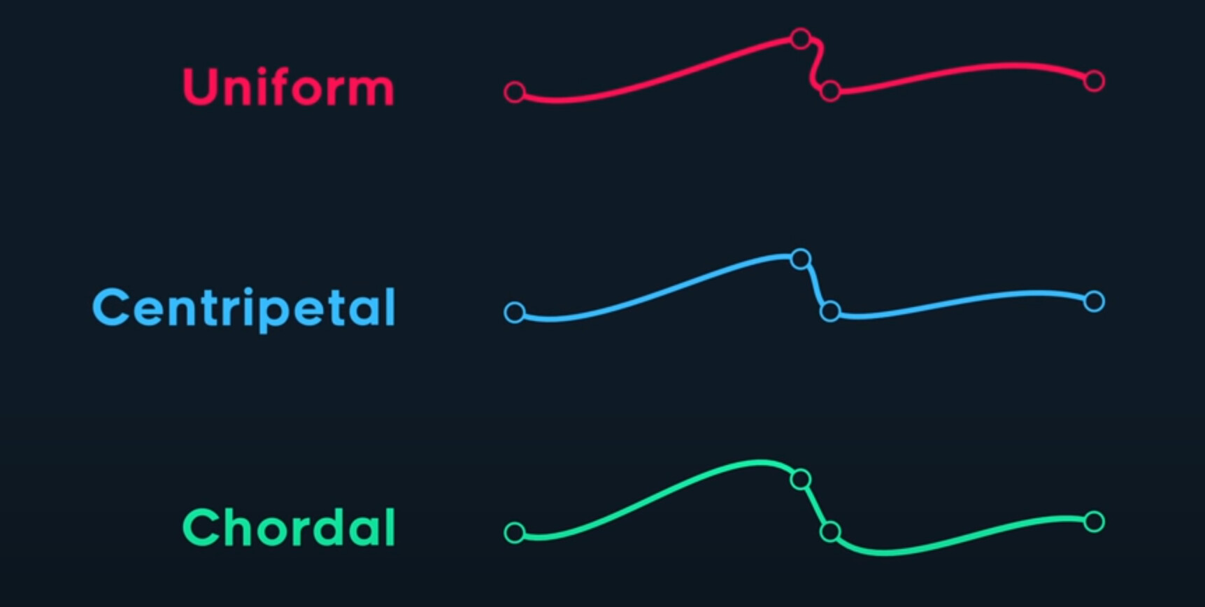
And while the uniform B-Spline we looked at earlier was useful in its own right, if we allow changing the time or knot values, we get the non-uniform B-spline. All the continuity promises of the B-spline are still intact, this in turn afects the shape of the spline, too.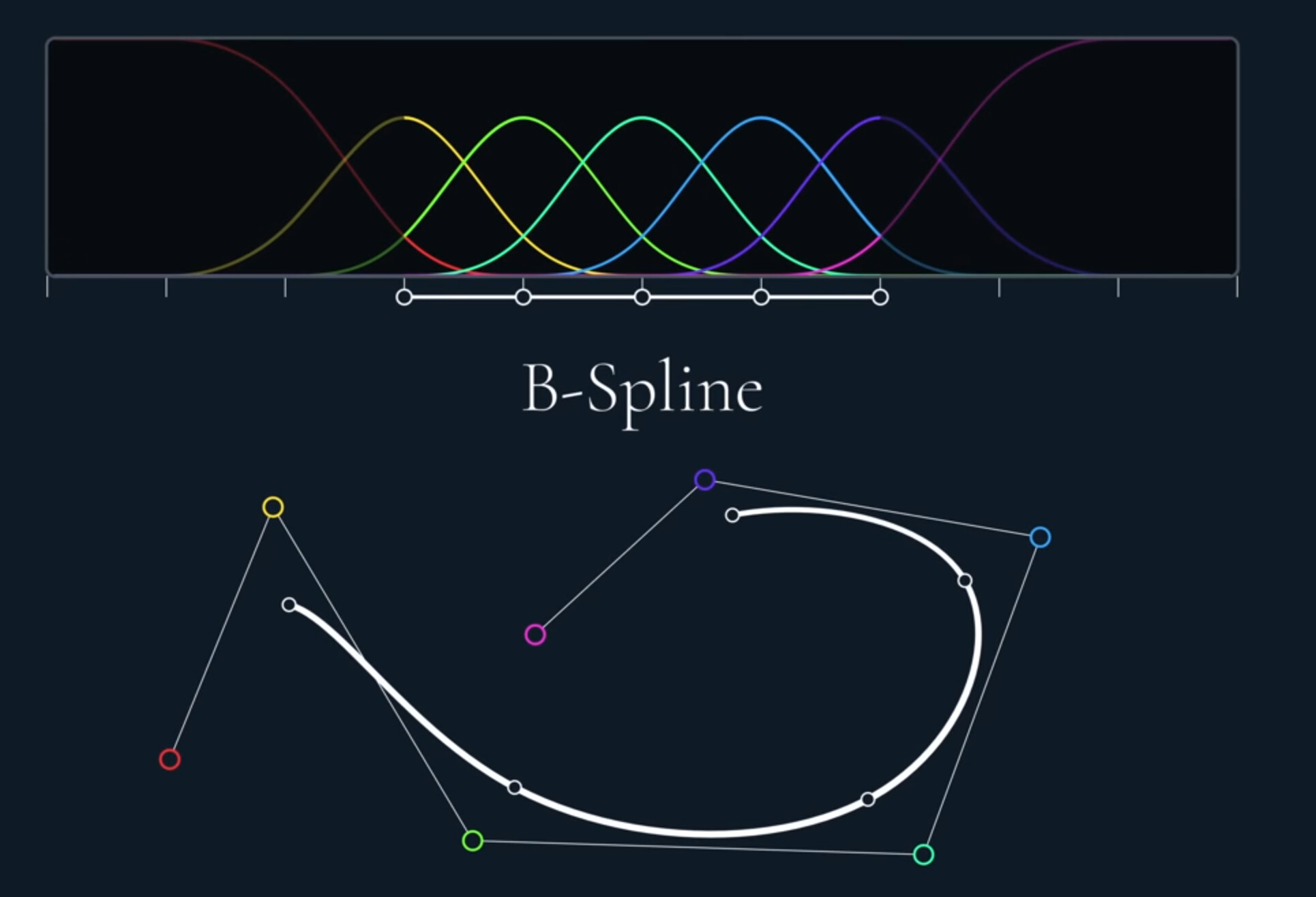
There’s an even more advanced variant, called the non-uniform rational B-spline, that lets you control the priority or weight of each control point, making the curves gravitaete toward or away from specific control points.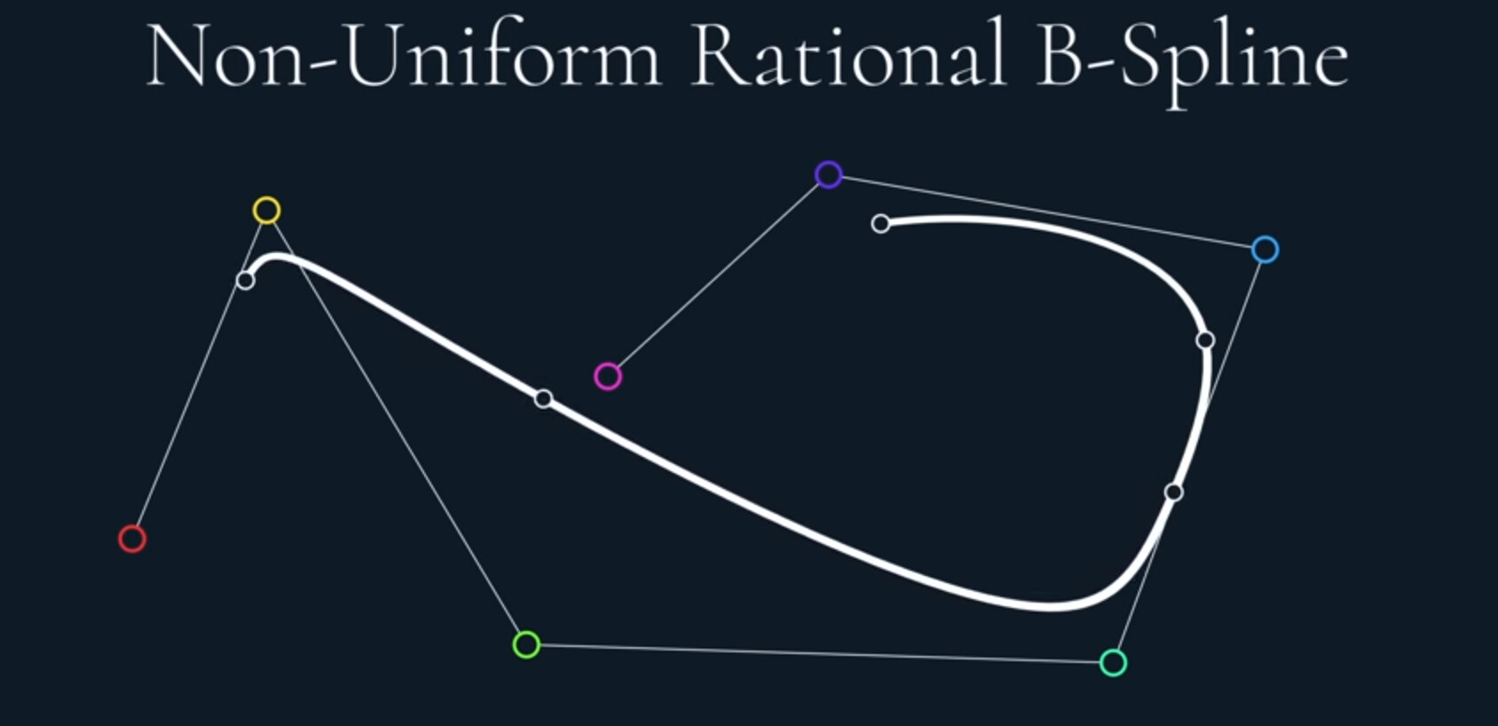
We might even have heard of this one before, it’s more commonly known by its short name–NURBS.
So every color key in a gradient, is a control point of linear spline, in color space. Then if we want to use this as a gradient map on an image, instead of using time as our input, we use the brightness of its pixels to sample the gradient. The output is then in full color, based on our color spline.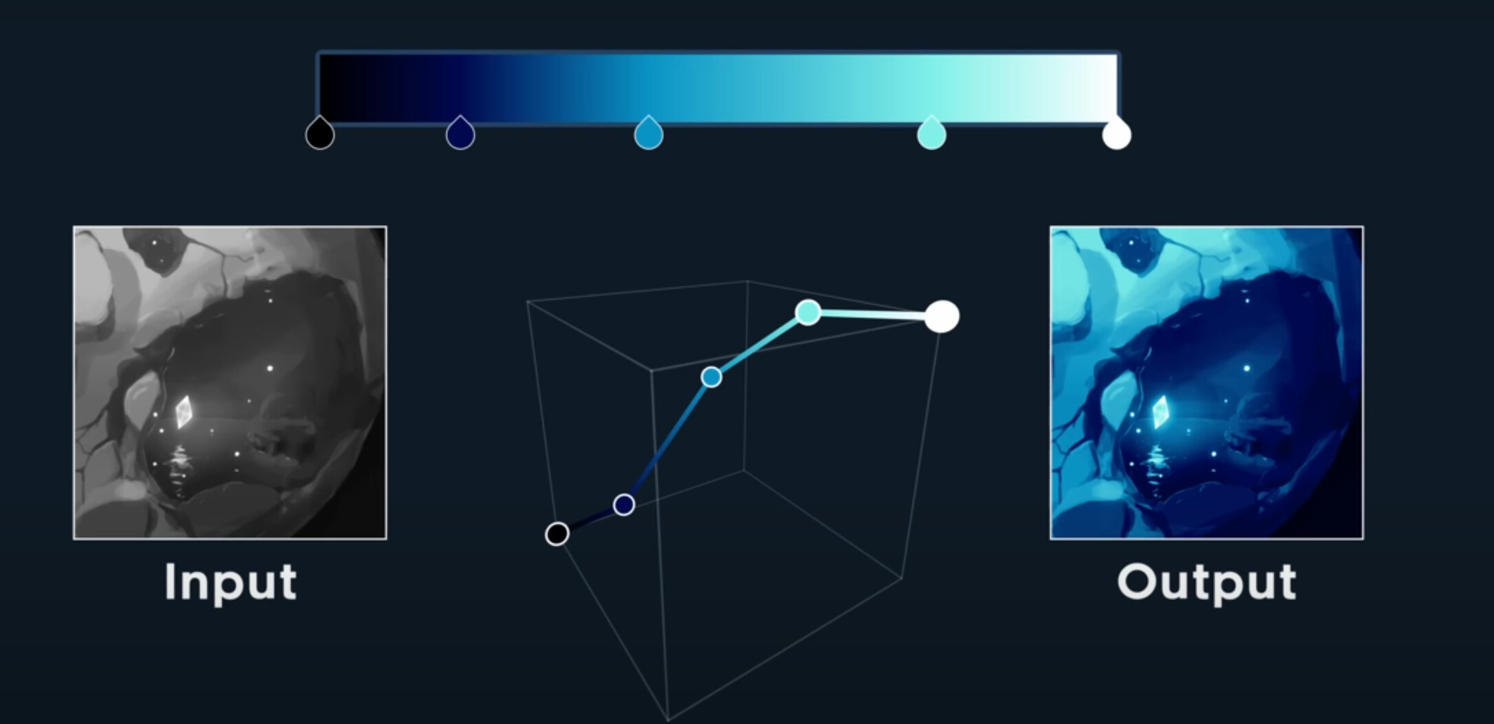
If we then move the control points, in other words, change the colors and time of our keys, the output changes along with it.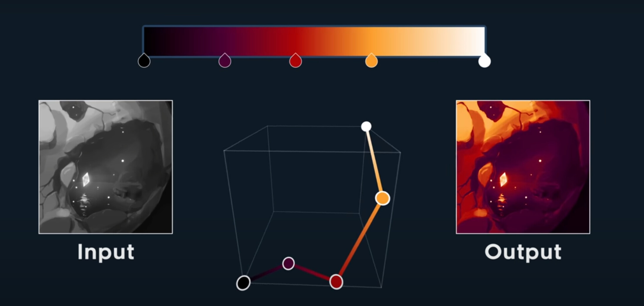
As you can see, splines show up in many, perhaps, unexpected places. The whole field goes much deeper than what we had time for today.
I hope you fouind this little exploration of math noodles interesting!
Thank you all so much for watching here!